

by Javier Vinós & Andy Might
“These shifts are related to vital modifications in world temperature pattern and in ENSO variability. The most recent such occasion is called the nice local weather shift of the Nineteen Seventies.”
Anastasios A. Tsonis, Kyle Swanson & Sergey Kravtsov (2007)
4.1 Introduction
Whereas the research of climate variability has a protracted custom, the science of local weather change is a really younger scientific subject, as attested to by the 1984 discovery of the primary multidecadal oscillation, the first world local weather inner variability phenomenon, by Folland et al. The impression of this basic function of the worldwide local weather system was found ten years later by Schlesinger and Ramankutty (1994), after fashionable world warming had already been blamed on CO2 modifications, illustrating the chance of reaching a consensus with inadequate understanding of the subject at hand. The Pacific (inter) Decadal Oscillation (PDO) was found three years later (Mantua et al. 1997; Minobe 1997). The Atlantic Multidecadal Oscillation (AMO) was not named till simply 20 years in the past (Kerr 2000).
Previous to the Eighties, it was typically thought that local weather modified so slowly as to be nearly imperceptible through the span of a human lifetime. However then it grew to become clear that abrupt local weather modifications occurred through the previous glacial interval (Dansgaard et al. 1984), Dansgaard–Oeschger occasions demonstrated that regional, hemispheric, and even world local weather may bear drastic modifications in a matter of many years. The issue was that fashionable climate-change idea was constructed round gradual modifications within the greenhouse impact (GHE) and didn’t have a lot room for abrupt, drastic, world modifications that would not be correctly defined by modifications in greenhouse gasoline (GHG) radiative forcing.
The primary explanations for glacial Dansgaard–Oeschger occasions concerned drastic modifications in meridional transport (MT) by the Atlantic Meridional Overturning Circulation (AMOC). AMOC is a part of the worldwide conveyor idea that tries to elucidate the move of warmth by means of the Earth’s oceans. The AMOC rationalization, higher generally known as the salt-oscillator speculation (Broecker et al. 1990), falls brief nonetheless, as there isn’t any proof that the AMOC has undergone the abrupt and drastic modifications required to supply the occasions. The present idea on MT is predicated on what is called the Bjerkness compensation speculation, the place modifications in one among MT elements (the oceanic or the atmospheric) are compensated for by comparable modifications of the other signal within the different. Present interpretations of the Dansgaard–Oeschger phenomenon are based mostly on fast sea-ice modifications happening within the Nordic seas that abruptly launched a large amount of ocean-stored warmth below the sea-ice (Dokken et al. 2013).
Dansgaard–Oeschger occasions have turned out to be a glacial-world phenomenon with little applicability to present Holocene situations, however it’s clear that abrupt local weather modifications are a actuality that requires a proof. Research of Holocene local weather change have recognized no less than 23 abrupt local weather occasions (Fig. 4.1e; Vinós 2022) through the previous 11,700 years (about two per millennium on common). They’re nicely mirrored in a number of proxies of various nature and recognized as such within the paleoclimatic literature. From their totally different climatic signatures, it’s clear that these occasions should not a response to a single trigger. But fashionable climate-change idea has left us with solely two potentialities, modifications in radiative forcing produced by modifications in atmospheric GHGs, or volcanic exercise. These easy processes can not clarify all of them. Adjustments in CO2 may be dominated out as a trigger, since from 11,000 years in the past to 1914 it remained between 250 and 300 ppm, and decadal to centennial oscillations in CO2 have solely assorted just a few ppm in keeping with ice cores. Volcanic forcing presents an issue, as a result of its Holocene evolution has been reverse to temperature evolution. It was stronger when the planet warmed and weaker when it cooled, reaching a minimal c. 3,000 years in the past, so it can’t be a powerful driver of centennial temperature change. In reality, the Little Ice Age (LIA), the latest abrupt local weather occasion previous to fashionable world warming, can’t be defined by CO2 or volcanic forcing. In accordance with the GISP2 ice core volcanic sulfate document (Fig. 4.1c; Zielinski et al. 1996), volcanic exercise was above common between 1166–1345 AD, however was beneath common throughout many of the LIA, solely turning into elevated once more in the direction of the top of it, within the 1766–1833 AD interval, because the world started to heat.

In Fig. 4.1, (a) is the black curve, a world temperature reconstruction from 73 proxies (after Marcott et al. 2013; with unique proxy dates and differencing common), expressed as the gap to the typical in normal deviations (Z-score). The purple curve, (b), is Earth’s axial tilt (obliquity) in levels. The purple curve (c) is the Holocene volcanic sulfate within the GISP2 ice core in elements per billion summed for every century within the BP scale (rightmost level is 0–99 or 1851–1950), with the quadratic trendline proven as the skinny purple line. Information are from Zielinski et al. 1996. Curve (d) is mild blue and exhibits CO2 ranges as measured within the Epica Dome C (Antarctica) ice core. Information are from Monnin et al. 2004. The sunshine gray bars, (e), are abrupt climatic occasions through the Holocene decided from ice-rafted petrological tracers (Bond et al. 2001), methane modifications (Blunier et al. 1995; Kobashi et al. 2007; Chappellaz et al. 2013), Useless Sea degree modifications (Migowski et al. 2006), δ18O isotope modifications in Dongge Cave (Wang et al. 2005), North Levant precipitation modifications (Kaniewski et al. 2015), and dolomite abundance modifications within the Gulf of Oman eolian deposition document (Cullen et al. 2000). Darkish gray bins at backside give their approximate dates in ka. The determine is from Vinós 2022
Trendy local weather idea has an issue explaining previous abrupt local weather modifications and has developed a obscure rationalization that makes use of ideas from chaos idea about thresholds which might be crossed and tipping factors which might be reached when a forcing progressively will increase over a loud chaotic background. The issue is that there isn’t any proof for the existence of such thresholds and tipping factors apart from the existence of the abrupt local weather modifications that they attempt to clarify. Theoretical optimistic feedbacks are additionally invoked, however the common local weather stability that has been life-compatible for the previous 450 Myr signifies that it’s a system dominated by adverse feedbacks. As is normally the case with a troubled paradigm, it takes refuge on the least identified elements of local weather, just like the significance of the poorly measured themohaline circulation for local weather change, discovering some help usually circulation fashions, however not on the observational proof, that implies AMOC is much more secure than beforehand thought (Worthington et al. 2021), and doesn’t seem to rely a lot on deepwater formation (Lozier 2012).
In addition to abrupt local weather occasions that occurred centuries or millennia in the past, present local weather additionally undergoes fast regime shifts each few many years. The regime shift idea was developed in ecology to elucidate fast transitions between different secure states, primarily in grazing ecosystems. Lluch-Belda et al. (1989) used the idea to elucidate the alternation between sardine and anchovy regimes concurrently in a number of of the world oceans, presumably in response to local weather change. Their information confirmed that no less than two shifts between sardine and anchovy regimes had taken place through the 20th century previous to the Eighties.
4.2 The local weather shift of 1976-77
On the 1990 7th Annual Pacific Local weather Workshop, Ebbesmeyer et al. (1991) introduced a research demonstrating that in 1976 the Pacific local weather had undergone a step change in 40 environmental variables, together with air and water temperatures, the Southern Oscillation, chlorophyll, geese, salmon, crabs, glaciers, atmospheric mud, coral, carbon dioxide, winds, ice cowl, and Bering Strait transport. The modifications recommended that one among Earth’s largest ecosystems sometimes undergoes abrupt shifts. Nicholas Graham (1994) analyzed the abrupt modifications that occurred within the boreal winter circulation over the Northern Hemisphere (NH) and within the coupled ocean/ambiance system of the tropical Pacific and concluded that these modifications resemble a muted, quasi-permanent El Niño, that started when the coupled ocean-atmosphere system didn’t get well totally from the 1976-77 El Niño and had been finest described as a change within the background local weather state. As well as, mid-latitude winter boreal circulation grew to become extra vigorous, with a southward tour of the westerlies, vital modifications in geopotential heights and sea degree stress, accompanied by a southward migration of the Aleutian low-pressure heart in winter.
Examination of previous local weather and fishery information from the North Pacific by Mantua et al. (1997) and by Minobe (1997) led to the identification of a 50–70-year local weather oscillation that was named the Pacific [inter] Decadal Oscillation (PDO; Mantua et al. 1997). Regime shifts within the PDO had been recognized in each articles c. 1925, 1947, and 1977. The pan-Pacific coordinated modifications in local weather and ecological variables had been obvious in lots of sea-surface temperature (SST) and sea-level stress (SLP) indices, just like the Southern Oscillation Index, outlined by Gilbert Walker within the Nineteen Twenties, and identified because the Sixties to trace atmospheric El Niño-linked modifications within the Walker circulation. Mantua and Hare outlined the PDO because the main principal part of an empirical orthogonal perform of month-to-month SST anomalies over the North Pacific (poleward of 20°N; Mantua & Hare 2002). As modifications in SLP lead modifications in SST by about two months, Shoshiro Minobe (1999) centered on SLP, utilizing the North Pacific Index (Trenberth & Hurrell 1994) that tracks seasonal SLP modifications in an ample area of the North Pacific centered on the Aleutian Low. Utilizing this index, Minobe confirmed that there have been two oscillations inflicting local weather shifts. The foremost oscillation, already recognized, had a interval of c. 55 years. It affected SLP variability throughout each winter and spring atmospheric circulation, and introduced shifts at c. 1922/23, 1948/49 and 1975/76 (Minobe 1999). The minor oscillation had a interval of c. 18 years, and solely affected winter circulation. Three intervals of the minor oscillation (i.e., shifts at c.1923/24, 1946/47 and 1976/77) almost coincide in time and signal with stress modifications of the most important oscillation (Fig. 4.2).
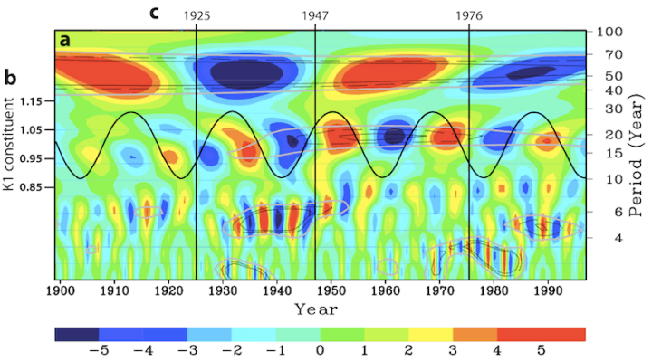
In Fig. 4.2, the central graph (a) is the wavelet-transform coefficient of the winter North Pacific index because the area-averaged sea-level stress anomaly (hPa) within the area 160°E−140°W, 30−65°N. It’s a three-dimensional illustration of the time area (1899–1997, X-axis), the frequency area (periodicity, Y-axis), and the amplitude of the modifications (shade scale, hPa) of the stress modifications in a area centered within the Aleutian Low. Blue shade signifies a deeper Aleutian Low related to PDO optimistic phases. The skinny black-solid, black-dashed and gray contours point out the importance on the 95, 90 and 80 % confidence ranges, respectively. The plot is from Minobe 1999. The thick black line, left scale, (b) is the part and amplitude sine wave of the diurnal lunar nodal cycle K1 tidal constituent. It has been overlain to point out that each the part and interval of the bidecadal part within the instrumental document is that of the 18.6-year lunar nodal cycle. The sine wave is after McKinnell and Crawford (2007). The dates of Pacific local weather regime shifts (c) are proven as vertical traces, as recognized by Mantua et al. (1997).
The North Atlantic additionally presents a multidecadal oscillation, the AMO, and a bidecadal one (Frankcombe et al. 2010). The connection between the bidecadal and multidecadal oscillations stays unclear. A subharmonic relationship is unlikely regardless of their coupling. Within the North Pacific they’ve a special seasonal dependency, and within the North Atlantic the bidecadal oscillation is finest seen in subsurface temperatures, whereas the multidecadal one impacts primarily floor temperature and Arctic deep-water salinity (Frankcombe et al. 2010). McKinnell and Crawford (2007) suggest that the North Pacific bidecadal oscillation is a manifestation of the 18.6-year lunar nodal cycle in winter air and sea temperatures. This lunar cycle strongly impacts the magnitude of the lunar diurnal tide constituent (K1) and is synchronized in part and interval to the bidecadal oscillation. In Fig. 4.2 rising K1 (upward sinusoidal) is related to lowering SLP (blue colours) and lowering K1 with rising SLP. In accordance with McKinnell and Crawford, the bidecadal part of variability affiliation to the 18.6-yr lunar nodal cycle seems in proxy temperatures of as much as 400 years in period. A tidal trigger for the bidecadal oscillation actually offers a proof for the subsurface temperature impact within the North Atlantic. Tides present over half of the power for the vertical mixing of water within the oceans.
The work of Schlesinger and Ramankutty (1994) made clear that multidecadal variability had impact on world temperature, which additionally shows a c. 55–70-year oscillation when detrended. Interdecadal oscillations have been described in most oceans, together with the Arctic, affecting a wide range of climatic phenomena together with SST, SLP, sea subsurface temperature, salinity, sea-ice, wind pace, sea-level, and atmospheric circulation. It was essential to take a world view integrating all this pure variability right into a single speculation of world multidecadal inner local weather change. That is what Marcia Wyatt completed when she developed the “stadium-wave” speculation in her thesis (Wyatt 2012). She recognized a multidecadal local weather sign that propagated throughout the Northern Hemisphere by means of the indices of a synchronized community (Fig. 4.3). Whereas Wyatt couldn’t establish the character of the sign, or the reason for its interval of c. 64 years, Wyatt and Curry (2014) recognized the Eurasian Arctic sea-ice area because the place the place the sign was first generated. As we noticed in Half III, that is the primary gateway for atmospheric winter meridional transport into the Arctic (e.g., see Figs. 3.6 & 3.8b), which may be very delicate to sea-ice.
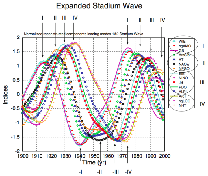
Fig. 4.3 exhibits the Twentieth-century sign propagation by means of a 15-index-member community. Chosen indices are a sub-set of a broader community. 4 clusters of indices are highlighted (I by means of IV, every may be optimistic or adverse). Every cluster is termed a “Temporal Group”. Peak values of Group indices signify phases of climate-regime evolution. The plot is from Wyatt and Curry 2014.
Clearly a hemispherically synchronized multidecadal variability within the ocean-atmosphere coupled system takes place within the NH throughout winter. Most fashionable world warming has additionally taken place since 1976 within the NH through the winter months (Fig. 4.4). It’s apparent to anyone endowed with impartial pondering that the local weather shift that affected the NH winters since 1976 and the worldwide warming that primarily affected the NH winters since 1976 have to be causally associated. On the very least, pure multidecadal variability have to be answerable for an necessary a part of the worldwide warming skilled within the 1976–2000 interval. But by the point multidecadal warming and local weather regime shifts had been identified to climatologists (within the Nineties–2010s), fashionable local weather idea had already performed a trump card assigning the 1976 local weather shift to aerosols. As Tsonis et al. write:
“The usual rationalization for the submit Nineteen Seventies warming is that the radiative impact of greenhouse gases overcame shortwave reflection results resulting from aerosols. Nonetheless, … the observations with this occasion, suggests another speculation, particularly that the local weather shifted after the Nineteen Seventies occasion to a special state of a hotter local weather, which can be superimposed on an anthropogenic warming pattern.”
Tsonis et al. (2007)
Regardless of figuring out this, fashionable local weather idea has refused to include the impact of local weather shifts, that are poorly reproduced and by no means predicted by fashions. This units the speculation up for failure as the identical trump card can’t be performed once more when the subsequent shift comes. Can the proponents of contemporary local weather idea ignore a brand new shift? Or will they acknowledge the speculation’s shortcomings, after committing western economies to a profound decarbonization?
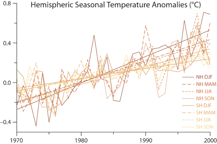
Fig 4.4 exhibits the Northern Hemisphere and Southern Hemisphere common temperature anomaly for December-February (steady), March-Might (lengthy sprint), June-August (brief sprint), and September-November (dotted) for the 1970–2000 interval. The information are from Jones et al. 2016.
4.3 Regardless of all of the individuals learning local weather, the 1997–98 shift went unnoticed
The failure to include local weather shifts to the trendy local weather idea is likely one of the causes the local weather shift that occurred in 1997–98 (97CS) was not seen and correctly described. One more reason is that lots of its results had been erroneously assigned to the rising radiative forcing from climbing GHGs ranges and used to boost the extent of local weather alarm. Because the 1976 shift modified the NH local weather to a hotter state (Tsonis et al. 2007) by rising the speed of warming (Fig. 4.4), the 97CS did the other and adjusted the local weather state by lowering the speed of warming. Embarrassingly, it was not local weather scientists who seen this variation, because it didn’t match their biases with regard to rising GHGs, but it surely was a geologist and paleontologist skeptical of contemporary local weather idea who first reported it:
“There IS an issue with world warming… it stopped in 1998”
(Carter 2006)
After the pause in world warming was recognized, tons of of articles had been revealed on it in scientific journals and an ideal controversy erupted over its actuality, with some authors denying its existence (Lewandowsky et al. 2016) and even altering the official datasets to scale back its significance (Karl et al. 2015), and different authors asserting it was an actual phenomenon that wanted a proof (Fyfe et al. 2016).
The pause controversy was a 3rd issue obscuring recognition of the 97CS regardless of clear proof of its existence. This issue, along with the absence of local weather shifts in fashionable local weather idea and fashions, and the wrong attribution of its results to rising GHG forcing, stored the apparent conclusion out of the mainstream. Lluch-Belda et al. (1989) recognized world sardine and anchovy regime shifts suggesting a local weather change trigger. These fishery shift factors had been later recognized as Pacific local weather shift factors that had world teleconnections (Mantua & Hare 2002). Chavez et al. (2003) reported within the journal Science {that a} new multidecadal regime shift in Pacific fisheries had taken place within the mid-Nineties. The nice and cozy “sardine regime” had modified to a cool “anchovy regime.” The authors suggested (clearly to no avail) that these large-scale, naturally occurring variations must be taken under consideration when contemplating human-induced local weather change. The 97CS continues to be unrecognized by local weather scientists. The following shift will most likely happen within the late 2020s to early 2030s. It could be shameful if local weather scientists, at the moment, are nonetheless unprepared for the change, and don’t acknowledge multidecadal variability contribution to fashionable world warming.
4.4 How the local weather shifted globally on the 97CS
Science is so specialised and compartmentalized lately that no one has pulled collectively all of the proof that confirms the 1997-98 world local weather shift. A shift that’s clearly unexplained by modifications in GHGs ranges and fashionable local weather idea. Photo voltaic exercise modified from excessive at photo voltaic cycle (SC) 22 to low at SC24 (Fig. 4.5a, black line). This modification may be higher appreciated within the nice lower within the antipodal amplitude magnetic index (Fig. 4.5a, purple line), that measures geomagnetic disturbances brought about primarily by the photo voltaic wind, to centennial low values. Now we have already talked about the well-known pause in world warming (Fig. 4.5b), that may be higher characterised as a discount within the fee of world warming after the mid-Nineties, and continues to be ongoing regardless of its interruption by the sturdy 2015–16 El Niño, after which no extra warming has taken place, as of the center of 2022.
On the 97CS, a predominantly Niño frequency sample in ENSO became predominantly Niña, as decided by the cumulative multivariate El Niño index (MEI v.2). The summed index confirmed an rising pattern through the earlier local weather regime, peaked in 1998, and exhibits a declining pattern after (Fig. 4.5c, black line). Heat water quantity on the equator decreased in variability (Fig. 4.5c, purple line), and strongly adverse anomalies within the heat water quantity, that used to occur as soon as a decade, stopped after 2000. A westward shift in atmosphere-ocean variability within the tropical Pacific occurred on the 97CS, characterised by a lower of ENSO variability that coincides with the suppression of subsurface ocean temperature variability and a weakening of atmospheric-ocean coupling within the tropical Pacific. The shift manifested as extra central Pacific versus japanese Pacific El Niño occasions, and a frequency improve in ENSO, linked to a westward shift of the placement of the wind-SST interplay area (Li et al. 2019). The modifications within the tropical Pacific atmospheric-ocean coupling had a mirrored image within the stratosphere. World (60°N-S) stratospheric water vapor decreased abruptly in 2001 (Fig. 4.5d). Concurrently, the tropical tropopause cooled (Randel & Park 2019), indicating {that a} step change within the tropical troposphere-stratosphere coupling additionally occurred.

Fig. 4.5 exhibits sequence that illustrate the massive climatic shift of 1997–98. Many almost simultaneous modifications in local weather associated phenomena occurred globally between 1995 and 2005. Panel (a) exhibits Oct–Jan sunspots (skinny black line) and the 11-yr common Oct–Jan sunspots (thick black line). Photo voltaic exercise decreased from excessive (108 sunspots 1980–1995) to low (54 sunspots 2005–2015). The information are from WDC–SILSO. The antipodal amplitude (Aa) geomagnetic index 13-month common is the skinny purple line, and the 11-year common is the purple thick line. The Aa geomagnetic index measures magnetic disturbances primarily attributable to the photo voltaic wind. The information are from ISGI. In panel (b) the worldwide floor common temperature anomaly in °C is plotted. It shows the 1998–2013 pause in warming. The information are from MetOffice HadCRUT 4.6 annual information. Panel (c) is the cumulative multivariate ENSO index v.2 as a black line. It modified from rising to lowering in 1998, indicating a shift within the ENSO sample. The information are from NOAA. The change can also be mirrored in a powerful discount within the heat water quantity anomaly (WWVa, proven in purple) variability on the equator (5°N–5°S, 120°E–80°W above 20 °C), the place after 2000 adverse values of minus one are now not reached. The information are plotted in 1014 m3 from TAO Venture Workplace of NOAA/PMEL. The stratospheric water vapor month-to-month anomaly at 60°N–S, 17.5 km peak, from photo voltaic occultation information (black line), and microwave sounder information (purple line) in ppmv are plotted in panel (d). The big drop in stratospheric water vapor in 2001 happens at about the identical time as a drop in tropical tropospheric temperature (not proven).
Panel (e) plots the cloud cowl anomaly, month-to-month as a skinny line, and yearly as a thick line. The anomaly is for 90°S–90°N cloud cowl in p.c. Information are from EUMETSAT CM SAF dataset, after Dübal & Vahrenholt (2021). Panel (f) is the ensemble imply annual Hadley cell depth anomaly (in p.c from the imply) for the NH from eight reanalyses (black line), and ensemble imply annual-mean Hadley cell edge anomaly (in levels latitude) for the NH from eight reanalyses (purple line). The plot is from Nguyen et al. 2013. Panel (g) is the typical annual change in length-of-day (ΔLOD) in millseconds, inverted (up is a shortening in LOD resulting from acceleration in Earth’s spin). The information are from IERS LOD C04 IAU2000A. Panel (h) is the yearly improve of the 10-year operating imply of the ocean warmth content material (black line), and the annual imply Earth power imbalance obtained because the distinction between the incoming photo voltaic radiation and the whole outgoing radiation (purple line). Each are in W/m2. The plot is after Dewitte et al. 2019. The illustration is from Vinós 2022.
On the 97CS, low cloud cowl decreased (Fig. 4.5e; Veretenenko & Ogurtsov 2016; Dübal & Vahrenholt 2021), and Earth’s albedo anomaly reached its lowest level in 1997 and began rising (Goode & Pallé 2007). The rise was resulting from rising excessive and center altitude cloud cowl. In the course of the 1995–2005 interval a tropicalization of the local weather occurred and the tropics expanded because the Hadley cells elevated their extent and depth (Fig. 4.5f; Nguyen et al. 2013). The atmospheric angular momentum decreased inflicting the pace of rotation of the Earth to extend, lowering the size of the day by 2 milliseconds (Fig. 4.5g). All these modifications altered the energetics of the local weather system. The Earth’s power imbalance, the incoming photo voltaic radiation minus the whole outgoing longwave radiation (OLR) as measured by the CERES system, began to lower, (Fig. 4.5h, purple line; Dewitte et al. 2019). The worldwide power change on the 97CS resulted in a change in pattern within the ocean warmth content material (OHC) time spinoff (Fig. 4.5h, black line; Dewitte et al. 2019). This modification signifies OHC began to extend extra slowly, which dismisses claims that the lacking warmth ensuing from the pause in warming was going into the oceans (Chen & Tung 2014).
These are a few of the world local weather variables that show a fast change at, or quickly after, the local weather regime shift recognized by Chavez et al. (2003) as a transition from a “heat” sardine to a “cool” anchovy regime, the other of the 1976 shift that was recognized within the Nineties. Twenty-five years after the popularity of local weather shifts, the 97CS nonetheless is just not acknowledged by fashionable local weather science. That the 76CS has been acknowledged and the 97CS has not is a powerful signal that fashionable local weather idea is an impediment to local weather change understanding and is inflicting scientists to dismiss info which might be inconsistent with their idea.
4.5 The Arctic shift and polar amplification
When the worldwide local weather shifted in 1997–98, the Arctic local weather was strongly affected. In Half III, when reviewing how warmth is transported through the winter to the Arctic, we talked about that little Arctic amplification had taken place by 1995 regardless of 20 years of intense warming, echoing the phrases of Curry and colleagues:
“The relative lack of noticed warming and comparatively small ice retreat might point out that GCMs are overemphasizing the sensitivity of local weather to high-latitude processes.”
Curry et al. (1996)
On the 97CS, Arctic amplification elevated significantly and all of a sudden, however displayed a hanging seasonality. Arctic summer season temperatures should not rising (Fig. 4.6a, black line). Any improve in web warmth transported in summer season to the Arctic is in an ideal half saved, by warming the ocean and melting ice and snow, till the arrival of the chilly season when it’s returned to the ambiance, by the reverse course of. Winter floor temperature exhibits a really pronounced improve since c. 1998 (Fig. 4.6a, purple line).
The impact of the 97CS on Arctic sea-ice extent was spectacular. Between 1996 and 2007 September Arctic sea-ice extent decreased by a whopping 45 % (Fig. 4.6b), resulting in fears amongst specialists that it had entered a death-spiral (Serreze 2010). However after 11 years of loses Arctic sea-ice tailored to the brand new regime and 14 years later September Arctic sea-ice extent was larger than in 2007. Since sea-ice loss was used as a poster youngster of enhanced greenhouse warming and Arctic amplification, and used to boost alarm and cash, it can not now be correctly attributed to the 97CS with out dropping face. The discount in Arctic sea-ice was accompanied on the 97CS by a rise in Greenland meltwater flux (Fig. 4.6c, black line), and a lower in Greenland ice-sheet mass steadiness (Fig. 4.6c, purple line), that show the identical dynamics of fast change within the years after the climatic shift adopted by a stabilization to the brand new regime ranges.

Fig. 4.6 exhibits the info traits of the massive Arctic climatic shift of 1997–98. Panel (a) exhibits the 80–90°N summer season (JJA, black line), and winter (DJF, purple line) temperature anomalies in °C. The information are from the Danish Meteorological Institute. Panel (b) exhibits the September common Arctic sea-ice extent (106 km2). The information are from NSIDC. Panel (c) is the Greenland freshwater flux (black line, km3). The information are from Dukhovskoy et al. 2019. The purple line is the Greenland ice-sheet mass steadiness in Gt, after Mouginot et al. 2019. Panel (d) is the Arctic Ocean Oscillation (AOO) index. It displays the alternation between sea-ice and ocean anticyclonic circulation (blue bars) and cyclonic circulation (purple bars). It’s after Proshutinsky et al. 2015. Panel (e) exhibits the variety of NH blocking occasions per 12 months, after Lupo 2020. Panel (f) is the winter (DJF) latent power transport throughout 70°N by planetary scale waves, in PW. The skinny line is the annual change, and the thick line is the 5-year shifting common. The plot is after Rydsaa et al. 2021. The illustration is from Vinós 2022.
Because the 97CS is unrecognized, scientists can not clarify most of the altered climatic parameters. That is true of the Arctic Ocean Oscillation index (AOO; Fig. 4.6d), outlined by Andrey Proshutinsky (2015) because the oscillation between cyclonic (anti-clockwise) and anticyclonic (clockwise) ocean circulation within the Arctic Beaufort gyre, with a interval of 10–15 years. The issue is that through the 97CS the oscillation stopped and the system obtained caught within the anticyclonic regime, which results in freshwater accumulation within the Arctic. 1996 was the final cyclonic AOO 12 months, as of late 2022. Proshutinsky has no rationalization and the index stopped being up to date in 2019, nonetheless he grew to become anxious that the rising Beaufort gyre freshwater accumulation is a “ticking time bomb” for local weather. The buildup might result in a salinity anomaly within the North Atlantic with a magnitude akin to the Nice Salinity Anomaly of the Nineteen Seventies, that traveled the sub-polar gyre currents from 1968 to 1982 and should have contributed to the early Nineteen Seventies cooling.
Extra unexplained modifications within the Arctic local weather on the 97CS embody the rise in winter blocking occasions, notably within the NH (Fig. 4.6e). We additionally reviewed, in Half III, how blocking situations cease the traditional westerly zonal circulation at mid-latitudes throughout winter. They’ve two excellent results. They stabilize climate patterns for days over the identical location, resulting in excessive climate occasions in temperature and precipitation; and so they additionally significantly improve MT in the direction of the Arctic since they deflect cyclones poleward. It’s clear, however not defined, that MT in the direction of the Arctic elevated on the 97CS, and that is the underlying reason for most of the modifications noticed afterward within the Arctic local weather. Proof for the rise in winter warmth and moisture transport into the Arctic comes from the rise in planetary-scale latent warmth transport (Fig. 4.6f), whereas synoptic scale latent warmth transport decreased throughout winters, however elevated throughout summers (Rydsaa et al. 2021). The rise in winter warmth and moisture transport into the Arctic results in larger cloud formation, which shifts the strongest radiative cooling from the floor to cloud tops, that are regularly hotter in winter resulting from temperature inversions. On the sea-ice border, winter warmth intrusions trigger a short lived retreat of the ice margin, resulting in enhanced warmth loss by the ocean till the ice varieties once more (Woods & Caballero 2016).
Arctic amplification has turned out to be primarily a chilly season phenomenon that began between 1995–2000 for causes unknown to most local weather scientists and fashions. Arctic amplification relies on modifications in MT, and the speed of Arctic amplification seems to be reverse to the speed of world warming.
4.6 Local weather regimes as a meridional transport phenomenon affecting planetary energetics
From the consequences of local weather shifts it’s evident that they have an effect on the worldwide MT system, and notably the boreal winter MT. As we reviewed in Half III, ENSO is a approach of extracting surplus warmth from the deep tropics that exceeds the common oceanic transport system. On the 97CS this want decreases because the Brewer-Dobson circulation (BDC, the stratospheric MT) turns into extra energetic driving extra warmth out of the deep tropics, inflicting a cooling on the tropical tropopause that leads to extra stratospheric dehydration. Additionally, meridional wind circulation turns into stronger on the expense of zonal circulation leading to Earth’s rotation acceleration and Hadley cells enlargement. As meridional moisture transport to the poles is enhanced with the rise in meridional wind circulation, cloud cowl decreases within the low and mid-latitudes, and will increase within the Arctic.
Within the Arctic the consequences of local weather shifts by means of modifications in MT depth are much more evident. On the 97CS, MT to the Arctic was enhanced all 12 months spherical, however extra strongly through the chilly season. The rise in warmth and moisture advection from decrease latitudes leads to a discount in sea-ice cowl that augments ocean warmth loss, and will increase chilly season (however not summer season) floor temperature. The principle impact of winter warming is to extend the radiative loss to area. As we noticed in Half III, the Arctic in winter may be very particular by way of GHE. The ambiance is extraordinarily dry, so there may be little water vapor GHE. Cloud cowl can also be fairly low through the winter, and the rise in CO2 has the impact of accelerating radiation to area from hotter, larger CO2 molecules (van Wijngaarden & Happer 2020).
When there may be an intense intrusion occasion of moist heat air into the Arctic in winter the standard result’s a temperature inversion, and regardless of elevated downward longwave radiation, radiative cooling continues from the highest of the inversion or the clouds till the advected moisture is both precipitated or exported again to decrease latitudes. In essence, extra warmth transported to the Arctic within the winter should end in extra warmth misplaced to area. This conclusion contradicts one of many fundamental pillars of contemporary local weather idea that states that MT is just not a local weather forcing since horizontal transport doesn’t have an effect on the quantity of power inside the local weather system, and subsequently is just not a trigger for local weather change. That is essentially the most basic of the various errors of contemporary local weather idea, because it assumes the highest of the ambiance behaves equally by way of GHE in every single place. It doesn’t, because the GHE may be very weak on the polar areas, notably through the lengthy chilly season. Transporting extra warmth from a area of excessive GHE to a area of low GHE leads to extra warmth being misplaced on the high of the ambiance with no compensating achieve elsewhere. A change within the depth of MT in the direction of the winter pole leads to a change within the planet’s power funds as we’ve proven (Fig. 4.5h).
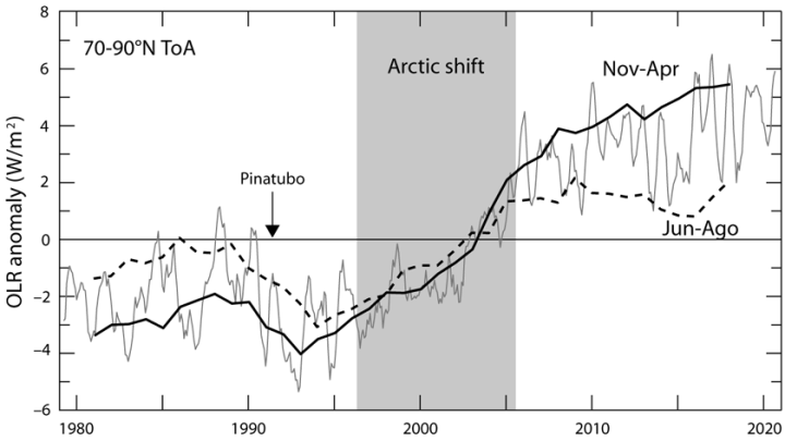
In Fig. 4.7 the skinny gray line is the 7-month common of the month-to-month imply OLR anomaly in W/m2 from the interpolated OLR NOAA dataset. The thick black line is the 5-year common of the chilly season (Nov–Apr) imply. The thick black dashed line is the 5-year common of the summer season (JJA) imply. The gray field highlights the Arctic shift in OLR between mid-1996 and late 2005. The time of the Pinatubo eruption is recognized. Information from KNMI explorer. The illustration is from Vinós 2022.
OLR within the Arctic is larger through the summer season than through the chilly season as may very well be anticipated from the close to everlasting summer season insolation and better floor temperature. Nonetheless, on the 97CS OLR elevated much more through the chilly season than through the summer season (Fig. 4.7). Clearly MT grew to become stronger, notably through the boreal winter. Elevated summer season transport resulted in additional power storage by means of enhanced summer season melting. Winter refreezing of the melted water returns the summer season power to the ambiance, solely to be misplaced to area by means of radiative cooling. Now we perceive why Arctic amplification is a winter phenomenon that’s not associated to world warming, and in reality is the place the power for the “Pause” goes. Arctic amplification is just not a GHG impact, however a MT impact that leads to planetary cooling. The pause is constant as a result of Arctic amplification is ongoing. When the pause ends the Arctic ought to cool and sea ice ought to develop. As said beforehand this might occur by late 2020s to early 2030s, when the subsequent local weather shift happens.
4.7 Meridional transport modulation of world local weather
To research the multidecadal modifications in MT since 1900, the 1912–2008 interval has been subjectively divided in three phases of 32 years. Though the totally different modes of variability don’t shift concurrently (therefore the title stadium-wave), the phases so outlined describe intervals of alternating prevailing situations in MT nicely. Beginning within the Arctic, the place the PV energy determines the polar stratosphere-troposphere winter coupling, the Arctic oscillation (AO; Fig. 4.8a, gray line) is the main mode of extratropical circulation variability within the NH (Thompson & Wallace 2000). To behave as a North-South seesaw of atmospheric mass alternate between the Arctic and mid-latitudes, the AO requires a correlation between its three facilities of motion —the Arctic, Atlantic and Pacific sectors. The Arctic-Atlantic correlation is called the North Atlantic Oscillation (NAO), and is robust, the Arctic–Pacific linkage is weaker, casting doubts in regards to the AO being a real annular mode. Nonetheless, the Aleutian Low and the Icelandic Low have had a adverse correlation from one winter to the subsequent because the mid-Nineteen Seventies (Honda & Nakamura 2001). This Aleutian–Icelandic seesaw seems to depend upon the propagation of stationary waves and varies in energy with modifications in PV energy (Solar & Tan 2013). By calculating the Jan–Feb cumulative AO (Fig. 4.8a, gray line) we are able to see that till c. 1940 optimistic AO values (i.e., sturdy vortex situations) prevailed, however within the 1940–Eighties interval adverse AO values had been extra frequent, solely to alter again afterwards. The Aleutian–Icelandic seesaw confirms the modifications in PV energy with its 25-year shifting correlation (Li et al. 2018; Fig. 4.8a black line). When the PV is robust, the mass and warmth alternate between the mid-latitudes and the Arctic is smaller, because the PV acts as a barrier to meridional circulation.
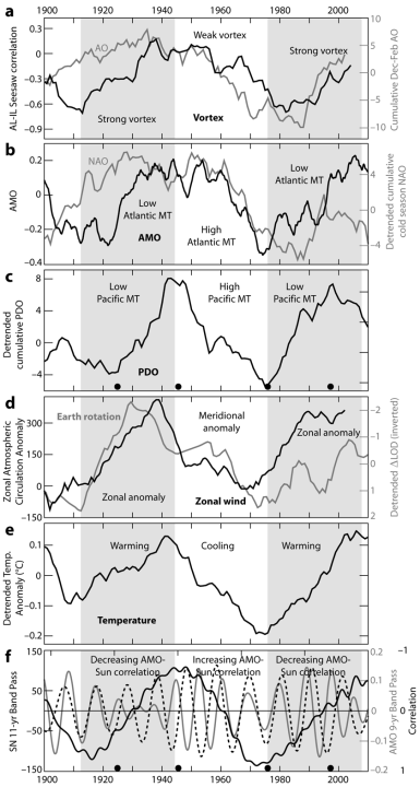
In Fig. 4.8, panel (a) exhibits the polar vortex energy. The black line is the Aleutian Low–Icelandic Low seesaw 25-year shifting correlation as a proxy for polar vortex energy. The plot is after Li et al. 2018. The gray line is the cumulative winter (Dec–Feb common) Arctic Oscillation index. The information are the 1899–2002 AO index from DW Thompson. Dept. of Atmos. Sci. CSU (Thompson & Wallace 2000). In panel (b), the black line is the 4.5-year common of the Atlantic Multidecadal Oscillation index. The information are from NOAA and unsmoothed from the Kaplan SST V2. The gray line is the cumulative 1870–2020 detrended chilly season (Nov–Apr common) North Atlantic Oscillation index. The information are from CRU, U. East Anglia, Jones et al. 1997. Panel (c) is the cumulative PDO. It’s the 1870–2018 detrended annual common cumulative PDO index from HadISST 1.1, and the info are from NOAA. The black dots mark the years 1925, 1946, 1976 and 1997 when PDO regime shifts occurred (Mantua & Hare 2002; see Sect. 11.4).
The black line in panel (d) exhibits the zonal atmospheric circulation index, cumulative anomaly. It’s after Klyashtorin & Lyubushin 2007. The gray line in panel (d) is the 1900–2020 inverted and detrended annual ∆LOD. The information is in milliseconds from IERS. Panel (e) is the detrended 1895–2015 annual world floor common temperature, 10-year averaged. The information are from Met Workplace HadCRUT 4.6. The panel (f) dashed line is the 8.2–16.6-year band-pass of the month-to-month imply complete sunspot quantity. The information are from WDC–SILSO. The gray line is the 6.6–11-year band-pass of the month-to-month AMO index. The black line is the inverted 20-year operating correlation of the band-pass sunspot and AMO information. The black dots point out local weather shifts, as in c, exhibiting their place with respect to photo voltaic minima. The illustration is from Vinós 2022.
The AMO measures SST anomalies that mirror the energy of MT over the North Atlantic. Optimistic AMO values point out heat water accumulation resulting from lowered MT and powerful PV situations (Fig. 4.8b, black line). The NAO is the sea-level stress dipole over the North Atlantic, and a part of the AO. Not surprisingly, its detrended and cumulative worth is similar to that of the AO, but in addition exhibits some correlation to the AMO SSTs (Fig. 4.8b, gray line). The decades-long NAO traits can’t be defined by common circulation fashions as they don’t incorporate multidecadal MT regimes. Fashions contemplate NAO indices white noise with out serial correlation (Eade et al. 2021). With out correctly representing MT, local weather fashions can not clarify local weather change. Over the Pacific sector, the PDO additionally measures SST anomalies. A optimistic PDO signifies heat water accumulation over the equatorial and japanese facet of the Pacific, a sign of lowered MT, which strikes warmth out of the equator and in the direction of the western Pacific boundary so the Kuroshio present can transfer it northward and switch it to the ambiance. The detrended cumulative PDO values (Fig. 4.8c) present that the phases of elevated or decreased Pacific MT roughly coincide with these of the Atlantic. Climatic and ecological shifts within the Pacific recognized in 1925, 1946, 1976 and 1997 (Mantua & Hare 2002) coincide with instances when the PDO shifts from predominantly optimistic to adverse or again (Fig. 4.8c black dots).
The meridional wind circulation is how many of the tropospheric MT is carried out and will increase in MT suggest will increase in meridional circulation and corresponding decreases in zonal circulation. The atmospheric circulation index is a cumulative illustration of the yearly anomaly in zonal (E–W) versus meridional (N–S) air-mass switch in Eurasia (Klyashtorin & Lyubushin 2007). Intervals when the NH PV has been stronger and MT over the North Atlantic and North Pacific sectors has been decrease (gray areas in Fig. 4.8) coincide with intervals characterised by predominant zonal-type anomalies, whereas intervals of weaker PV and better MT current predominant anomalies of meridional-type (Fig. 4.8d, black line). These persistent modifications in predominant atmospheric circulation patterns produce modifications within the switch of momentum between the ambiance and the stable Earth–ocean affecting the Earth’s rotation pace, measured as modifications within the size of day. Intervals of accelerating zonal circulation correlate with an acceleration of the Earth and a lower in ∆LOD (inverted in Fig. 4.8d, gray line) whereas intervals of lowering zonal circulation correlate with a deceleration of the Earth and a rise in ∆LOD (Lambeck & Cazenave 1976). Adjustments within the fee of rotation of the Earth combine world modifications in atmospheric circulation that help the worldwide impact of MT modifications. We should keep in mind at this level that modifications in Earth’s rotation fee reply to modifications in photo voltaic exercise (see Fig. 2.5).
Multidecadal modifications in MT are the reason for the multidecadal oscillation generally known as the stadium-wave, and all its manifestations. SST modifications within the AMO and PDO are a response to modifications in world atmospheric circulation. A discount in atmospheric meridional circulation and the corresponding improve in zonal circulation imply much less poleward power transport, and since annual incoming power is close to fixed and ocean warmth transport is barely partially depending on wind-driven circulation, extra warmth accumulates at every latitudinal band, however notably within the NH mid-latitudes. It’s because sea floor switch of power and moisture to the ambiance is highest at NH mid-latitude ocean western boundaries (Yu & Weller 2007). Land and sea floor warmth accumulation ensuing from a discount in MT produces the stadium-wave results and a rise within the world temperature. When the worldwide common floor temperature anomaly is detrended, intervals of lowered (elevated) MT correspond to warming (cooling) with respect to the pattern (Fig. 4.8e). The trendy local weather idea explains the 1940–1975 hiatus as resulting from a rise in aerosols, and the 1976–2000 warming as because of the improve in anthropogenic emissions. These explanations, included into local weather fashions, are untenable in mild of the proof (Tsonis et al. 2007). Though an anthropogenic warming pattern is unquestionable, it’s evident that the shifts in MT regimes dominate the floor temperature response.
The causes behind the multidecadal stadium-wave modifications in MT are unknown. The c. 65-year oscillation is non-stationary. Proxy reconstructions point out that the AMO had a shorter periodicity and fewer energy through the LIA and an extended periodicity and extra energy through the Medieval Heat Interval (Chylek et al. 2012; Wang et al. 2017). Photo voltaic exercise modulation of ENSO and Earth’s rotation modifications had been proven in Half II (Figs. 2.4 & 2.5). As each are a manifestation of MT energy, it’s doable that inner variability and exterior photo voltaic forcing are answerable for the present periodicity and energy of the stadium-wave. Alternatively, inner variability in MT could be responding to the warming pattern imposed by anthropogenic and pure causes, primarily the rise in photo voltaic exercise related to the trendy photo voltaic most. The 4 local weather shifts recognized within the Pacific through the Twentieth century (Mantua & Hare 2002) occurred 1–3 years after a photo voltaic minimal (Fig. 4.8c & f, dots; photo voltaic cycle, Fig. 4.8f dashed line), and the 2 gray areas and center white space in determine 4.8, representing alternating MT regimes, span three photo voltaic cycles between photo voltaic minima. It has been proven that the Holton–Tan impact (see Half I), that relates the tropical QBO part to the energy of the PV, by means of planetary wave propagation, is stronger at photo voltaic minima (Labitzke et al. 2006), and that the Holton–Tan impact weakened considerably through the 1977–1997 interval of lowered MT (Lu et al. 2008). This suggests that in winter at photo voltaic minima the stratospheric tropical-polar coupling, and the stratospheric-tropospheric coupling are stronger, and so they would possibly represent an acceptable time for a coordinated shift in MT energy that takes impact through the ensuing photo voltaic cycle. We will see if future local weather shifts additionally happen instantly following photo voltaic minima. That is the idea of our projection that the subsequent local weather shift may happen round 2031–34.
If photo voltaic minima are the instances when MT shifts happen, one fascinating correlation might present a proof for the reason for the c. 65-year oscillation pacing. The AMO has a 9.1-year sturdy frequency peak that can also be discovered within the PDO (Muller et al. 2013). This frequency is instantly appreciated in a 4.5-year averaged AMO index as decadal bumps (Fig. 4.8b, black curve). The origin of this conspicuous AMO trait has not been adequately researched, however Scafetta (2010) convincingly proposes a lunisolar tidal origin. The distinction in frequency between this reported 9.1-yr tidal cycle and the 11-yr photo voltaic cycle is such that they modify from correlated to anti-correlated (i.e., constructive to damaging interference) with a periodicity that not solely matches the AMO, however is precisely synchronized to it (examine black curves in Fig. 4.8b & f). One can speculate {that a} constructive or damaging interference between the impact of oceanic and atmospheric tides on the tropospheric part of MT and the impact of the photo voltaic cycle on the stratospheric part of MT would possibly end result within the periodical change in MT energy that produces the noticed climatic shifts. In help of this speculation two intrinsic elements of c. 4.5 and 11 years are discovered within the Fourier evaluation of the each day NAO autocorrelation sequence (Álvarez–Ramírez et al. 2011). The 11-year part is part synchronized to the photo voltaic cycle besides throughout photo voltaic minima, indicating that NAO predictability will increase with photo voltaic exercise, and have become strongly anti-correlated through the 1997 photo voltaic minimal, when the 97CS occurred. A c. 65-yr local weather oscillation that depends upon photo voltaic exercise would clarify each the modifications in depth and periodicity over the past centuries as photo voltaic exercise has been altering. Its 20th century depth and periodicity are the results of the trendy photo voltaic most, and the non-stationarity of the pure multidecadal oscillation could be linked to photo voltaic exercise multidecadal variability.
It may be argued that multidecadal oscillations within the local weather system ought to common to zero over a number of intervals. Equally, different elements identified to have an effect on MT, just like the QBO and ENSO common to zero in comparable or shorter timeframes. Nonetheless, AMO reconstructions present that its values and amplitude have elevated significantly over the past two cycles, since about 1850 (Moore et al. 2017). This modification within the c. 65-year oscillation means that MT is necessary in fashionable world warming, because it coincides with the sturdy melting of glaciers and improve in sea-level rise that began round 1850 and precedes the sturdy improve in CO2 emissions after 1945 (Boden et al. 2009). Photo voltaic exercise impacts MT and doesn’t common to zero even in very lengthy timeframes as a result of it presents centennial and millennial cycles (Vinós 2022). There was a long-standing scientific debate about whether or not there is a vital impact of photo voltaic exercise on local weather. Sunspot data present that the typical variety of sunspots elevated by 24% from the 1700–1843 to the 1844–1996 interval (see Fig. 1.6). Photo voltaic variability is clearly concerned in MT variability (see Half II). The impact that photo voltaic variability has on MT, and the impact that MT has on the planet’s power imbalance (Figs. 4.5h & 4.7) settles the controversy on the photo voltaic exercise impact on local weather.
Within the subsequent a part of this sequence, the speculation of how photo voltaic variability impacts MT shall be introduced. It has been named the Winter Gatekeeper speculation as a result of photo voltaic exercise modulates the quantity of warmth that’s transported to the poles in winter, and thru it the planet’s power funds, constituting the primary local weather change modulator on centennial to millennial timescales, as recommended by paleoclimatological proof.
This submit initially appeared on Judy Curry’s web site, Local weather, And so forth.
