

by Javier Vinós & Andy Might
“The sophisticated sample of sun-weather relationships undoubtedly wants a lot additional clarification, however progress on this area can be hindered if the view prevails that such relationships shouldn’t be taken severely just because the mechanisms concerned in explaining them are usually not but recognized.”
Joe W. King (1975)
2.1 Introduction
As proven in Half I of this collection, the early Eighties noticed a reversal within the consensus about an essential sun-weather impact and finding out the subject was discouraged. The adversarial tutorial atmosphere resulted in only a few scientists dedicating their analysis efforts to this topic. Regardless of the difficulties, essential advances have been made concerning the sun-climate impact. Lack of curiosity and disrespect for a competing local weather change mechanism speculation by mainstream climatologists has resulted in these advances being ignored. They continue to be under-cited and unknown to most supporters and skeptics of the CO2 speculation. Extra importantly, they aren’t mentioned in most local weather papers, they’re merely ignored.
These advances check with local weather phenomena that sometimes are usually not correctly included in local weather fashions attributable to lack of expertise of how they occur or what causes them. They don’t seem to be, or solely weakly, reproduced by fashions, but most often they are often detected in local weather reanalyses the place the fashions are constrained by an enormous variety of actual observations.
Importantly, no speculation for a sun-climate impact may be appropriate if it can not clarify or accommodate the connection between these phenomena and photo voltaic variability. The sun-climate relationship, at current, represents a black gap in fashionable climatology that retains rising with out anyone seeing inside it.
2.2 Results on temperature and paleoclimatology
Paleoclimatology is the one subfield in climatology the place a perception in an essential sun-climate impact is taken into account. It’s because the information obtained from proxy local weather data of the Holocene typically show a transparent affiliation with photo voltaic exercise knowledge obtained from proxy photo voltaic data. When considered one of us (JV) researched the climatic results of the 2500-yr sun-climate cycle found by Roger Bray in 1968 (Fig. 2.1), he shortly discovered 28 articles finding out proxies that clearly displayed this cycle (Vinós 2022). Of these, 16 (57%) explicitly state that modifications in photo voltaic exercise are seemingly the reason for the noticed climatic modifications, and just one explicitly guidelines the photo voltaic connection out. We’re speaking about profound world climatic modifications of the distant previous, comparable in magnitude to the Little Ice Age (LIA) or fashionable world warming. Most paleoclimate researchers finding out them conclude they had been attributable to modifications in photo voltaic exercise. Fashionable climatology can not clarify them since they came about at instances when greenhouse gasoline radiative forcing modified little or no.
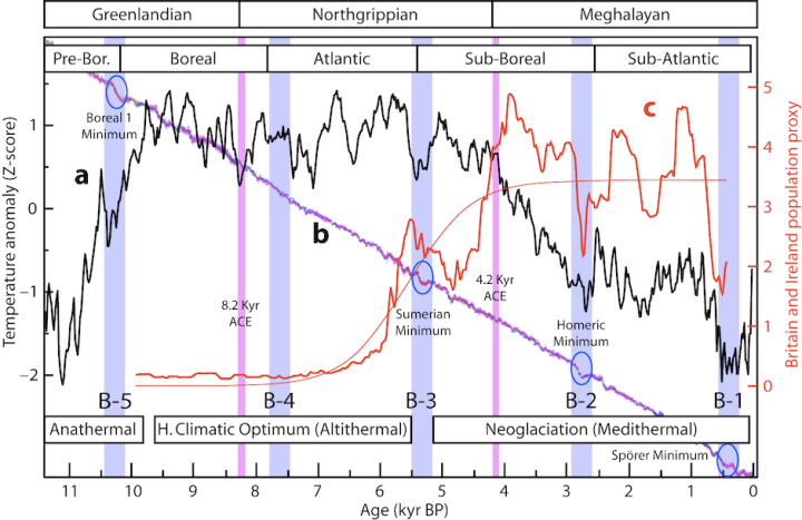
In Fig. 2.1 the foremost Holocene subdivisions are labeled. The stratigraphic subdivisions are on prime. The organic subdivisions are instantly under, displaying a c. 2500-yr spacing (after Ammann & Fyfe 2014). Classical subdivisions based mostly on temperature are throughout the underside. The black curve labeled (a) is a worldwide temperature reconstruction from 73 proxies (after Marcott et al. 2013; utilizing authentic proxy dates and differencing common), expressed as distance to the common in customary deviations (Z-score). The black curve and the labels present the foremost local weather modifications in the course of the Holocene. The blue/purple curve labeled (b) is the IntCal13 radiocarbon calibration curve used to transform radiocarbon dates (vertical, axis not proven) into calendar dates (horizontal). The blue/purple curve reveals the foremost photo voltaic modifications in the course of the Holocene, they’re after Reimer et al. (2013). The curve deviates from linearity throughout photo voltaic grand minima.
The Spörer, Homeric, Sumerian and Boreal 1 grand minima (blue ovals) are separated by multiples of c. 2500-yr, marking the lows of the Bray photo voltaic cycle B-1 to B-5, besides B-4. These lows have been recognized in radiocarbon knowledge again to B-9 at 20,500 BP (Vinós 2022). Human inhabitants knowledge is proven by (c), the purple thick curve, a summed likelihood distribution of anthropogenic radiocarbon dates from Britain and Eire as a proxy for human inhabitants. The purple skinny curve is a fitted logistic mannequin of inhabitants development and plateau, after Bevan et al. (2017). Vital draw back inhabitants deviations usually match the lows of the 2500-year Bray cycle of photo voltaic exercise (vast vertical blue bars labeled B-1 to B-5). The vertical pink bars are the 8.2 and 4.2 kyr abrupt climatic occasions (ACE).
The 2500-yr sun-climate Bray cycle constitutes a superb instance of the results of photo voltaic variability on paleoclimatology, because it produces essentially the most dramatic local weather cycle noticed within the Holocene. When it comes to photo voltaic exercise, it’s outlined by a sequence of Spörer-type grand photo voltaic minima that final 200 years and show a 20‰ improve in radiocarbon, spaced at 2500 ± 200 years with solely a niche at c. 7,700 BP within the final eight intervals since 20,500 BP (Fig. 2.1b; Vinós 2022). When it comes to local weather all of the lows of the cycle are marked by intervals of extreme local weather deterioration lasting over a century and mirrored in a number of proxies, of which the LIA constitutes the newest and the coldest instance in the course of the Holocene (Fig. 2.1a). When it comes to the results on human societies of the previous, the Bray cycle lows are marked by intervals of upheaval, inhabitants lower (Fig. 2.1c), and civilization collapse, adopted by societal advance afterward in response to a tough scenario.
The correspondence between previous photo voltaic exercise and previous local weather on the centennial and millennial timescales has brought on authors like Rohling to say:
“In view of those findings, we name for an in-depth multi-disciplinary evaluation of the potential for photo voltaic modulation of local weather on centennial scales.”
Rohling et al. (2002)
Magny et al. write:
“On a centennial scale, the successive climatic occasions which punctuated your complete Holocene within the central Mediterranean coincided with cooling occasions related to deglacial outbursts within the North Atlantic space and reduces in photo voltaic exercise in the course of the interval 11700–7000 cal BP, and to a doable mixture of NAO-type circulation and photo voltaic forcing since ca. 7000 cal BP onwards.”
Magny et al. (2013)
Hu et al. specific:
“Our outcomes indicate that small variations in photo voltaic irradiance induced pronounced cyclic modifications in northern high-latitude environments. In addition they present proof that centennial-scale shifts within the Holocene local weather had been comparable between the subpolar areas of the North Atlantic and North Pacific, probably due to Solar-ocean-climate linkages.”
Hu et al. (2003)
These three articles, between them, have 50 co-authors, amongst them a few of the most revered in paleoclimatology. Both the present understanding of the sun-climate impact or the present understanding of paleoclimatology is mistaken, as they’re incompatible. In science when unsure go along with the proof. Paleoclimatology has the proof, whereas the present consensus on the drivers of local weather change is predicated on laptop fashions that mirror programmers’ ignorance and biases.
The rise in photo voltaic irradiance in the course of the 11-yr cycle is about 1.1 W/m2. The anticipated floor warming for such a change in vitality is simply 0.025 °C and subsequently under detection (Wigley & Raper 1990). Temperature knowledge and reanalysis persistently present that the photo voltaic sign in world temperature is c. 0.1 °C, 4 instances bigger than anticipated from the vitality change alone (Lean 2017) thus the necessity to discover amplifying mechanisms. A really small vitality improve from the solar is predicted to lead to a really small evenly distributed temperature change on the floor. This isn’t what’s noticed. The change in floor temperature manifests itself in an unexplained, however important, regional and hemispheric variation and a few areas cool when extra vitality is coming from the solar (Fig. 2.2). These variations can solely be attributed to important dynamic modifications within the ambiance and oceans when the photo voltaic output varies by solely 0.1%.
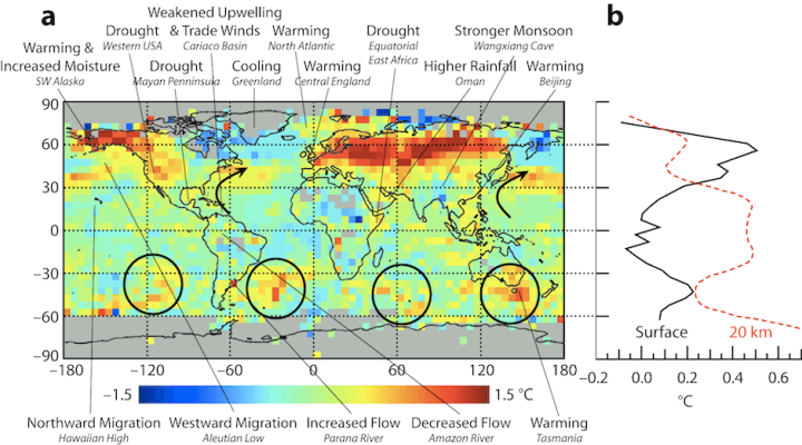
Fig 2.2, (a), is a floor temperature change map in the course of the 11-year photo voltaic cycle on a 5×5° grid from the 1996 photo voltaic minimal to the 2002 photo voltaic most utilizing a number of regression. A sample of discontinuous Southern Hemisphere mid-latitude warming is indicated by circles. The principle western boundary currents within the Northern Hemisphere are proven by black arrows. Examples of long-term local weather change responses to growing photo voltaic exercise obtained from paleo proof or lengthy local weather data are labeled at their areas. Zonally averaged change in floor (b, black line) and 20 km peak (b, purple line) temperature, with out a cosine space adjustment for latitude, after Lean 2017.
Whereas the worldwide common floor temperature improve with the photo voltaic cycle is simply 0.1 °C, at 60°N it reaches 0.4 °C (above 1 °C at some areas). This common sample of elevated floor warming within the Northern Hemisphere extra-tropics and decreased warming within the tropics and Southern Hemisphere produced by growing photo voltaic exercise isn’t not like the noticed floor warming over the previous 50 years. The floor temperature impact over North America confirms Currie’s (1993) discovering that the photo voltaic impact on temperatures is reverse on each side of the Rocky Mountains (see Half I). One other characteristic of photo voltaic induced warming is a sample of alternating Southern Hemisphere (SH) mid-latitude warming and minimal change or cooling with a spacing of c. 7000 km (Fig. 2.2a circles). They’re a tropospheric-ocean phenomenon and are extra conspicuous at 5 km altitude (see Lean 2017) and possibly mirror the worldwide wavenumber-4 atmospheric wave whose significance for SH local weather has been lately noticed (Chiswell 2021).
This photo voltaic modulated atmospheric wave-train phenomenon may very well be associated to the baroclinic annular mode (Thompson & Barnes 2014). Because the ambiance is intrinsically unstable, large-scale periodic atmospheric variability may be very uncommon exterior the tropics, as most atmospheric phenomena show purple noise traits. One of many few examples is the baroclinic annular mode, a 25–30-day oscillation within the SH extratropical eddy kinetic vitality related to variations within the amplitude of vertically propagating waves, that has essential results on regional local weather. The robust periodicity within the baroclinic annular mode, that coincides with the photo voltaic rotation interval, along with the wavenumber-4 sample over the 11-yr photo voltaic cycle, are suggestive of the baroclinic annular mode being modulated by modifications in photo voltaic exercise.
Lon Hood demonstrated that photo voltaic UV peaks modulate the Madden–Julian Oscillation. Day by day modifications in Madden–Julian Oscillation amplitude are modulated by UV modifications, because the amplitude will increase following UV minima. This amplitude modulating impact is larger in the course of the winter and spring and is strongest in the course of the easterly section of the Quasi-Biennial Oscillation (Hood 2018). On condition that the photo voltaic rotation interval is shut to at least one month, within the 4 photo voltaic cycles for which there’s satellite tv for pc knowledge there are c. 500 photo voltaic rotations, permitting a a lot better statistical analysis of this short-term photo voltaic impact on local weather.
One other characteristic of the floor temperature sample related to the photo voltaic cycle is the warming displayed on the extra-tropical western boundary currents, notably within the NH (Fig. 2.2a, black arrows). These are the popular websites for transferring vitality from the ocean to the ambiance (Yu & Weller 2007). The incoming vitality distinction related to the photo voltaic cycle may be very small, however the change in ocean-atmospheric vitality flux at these websites means that oceanic-atmospheric dynamic processes are regulated by modifications within the photo voltaic cycle. Lastly, the floor temperature sample is basically the reverse of the near-tropopause (20 km; Fig. 2.2b) sample, besides at NH excessive latitudes. Floor temperature modifications are usually not the results of direct modifications in TSI, since they’re regionally very various and 4 instances larger than the TSI vitality price range permits. This means that the contrasting floor and tropopause zonal temperature patterns come up from troposphere-stratosphere coupling.
Not solely the floor, but additionally the higher ocean shows a puzzling quasi-decadal change in temperature of c. 0.1 °C. White et al. (2003) analyzed the worldwide tropical diabatic warmth storage price range and located that the anomalous heating of the higher layer of the ocean to the depth of the 22°C isotherm yielded a worth of ± 0.9 W/m2, that’s almost an order of magnitude bigger than the floor radiative forcing of ± 0.1 W/m2 related to the photo voltaic cycle (photo voltaic radiative forcing is ΔTSI/4 x 0.7). Much more, the quasi-decadal temperature change within the higher ocean is phase-locked to the photo voltaic cycle, one thing that fashionable climatology can not clarify.
The close to whole lack of curiosity by fashionable climatologists within the sun-climate impact neglects the ample proof from paleoclimatology and up to date local weather variations that correlate with the solar-cycle. This reveals our poor information of the photo voltaic impact on local weather change. We’re all born ignorant, however some scientists select to stay so concerning the sun-climate query.
2.3 Results on the polar vortex
As reviewed in Half I (Sect. 1.6), it has been recognized since 1980 that the QBO modulates the power of the polar vortex (Holton & Tan 1980). Seven years later, Labitzke (1987) found that modifications in photo voltaic exercise affected this modulation. It was the primary strong, indeniable and climatically related sun-climate impact present in a 180-year-old quest. It additionally defined why the search had been so tough, because the impact is non-linear (not proportional to the full irradiance distinction) and oblique, relying on the route (QBO section) and power of the equatorial stratospheric winds.
The North Pole stratospheric temperature that Labitzke measured displays the state of the polar vortex. A powerful polar vortex is surrounded by robust winds, maintaining inside an space of low strain, low geopotential peak (peak of a given strain), and low temperature attributable to radiative cooling. Increased temperatures denote a weaker and/or displaced polar vortex. When the polar vortex turns into weaker and/or displaced in the course of the winter (i.e., larger North Pole stratospheric temperature), hotter air enters the Arctic, pushing the colder air under in the direction of decrease latitudes. A hotter North Pole with a weaker polar vortex signifies extra extreme winters in mid-latitudes. A better frequency of colder winters in northern mid-high latitudes was a characteristic of the LIA.
Labitzke’s knowledge confirmed that stratospheric North Pole temperature correlation to photo voltaic forcing is determined by QBO state. Throughout easterly QBO years stratospheric polar temperature is lowest when photo voltaic exercise is highest, and highest when photo voltaic exercise is lowest. The alternative happens throughout westerly QBO years (Fig. 2.3a). For the reason that lowest easterly-year and highest westerly-year temperatures are comparable, the biggest temperature variations for the 2 totally different QBO states happen throughout photo voltaic minimal years. The common winter North Pole stratospheric temperature distinction between each QBO phases throughout photo voltaic minima is an astounding 20 °C (Fig. 2.3b). The winter climatic impact of low photo voltaic exercise over ample areas of the North Hemisphere is clearly disproportionate to the full irradiance vitality distinction. A distinction that turns into irrelevant over the North Pole in the course of the boreal winter, when it’s in fixed darkness.
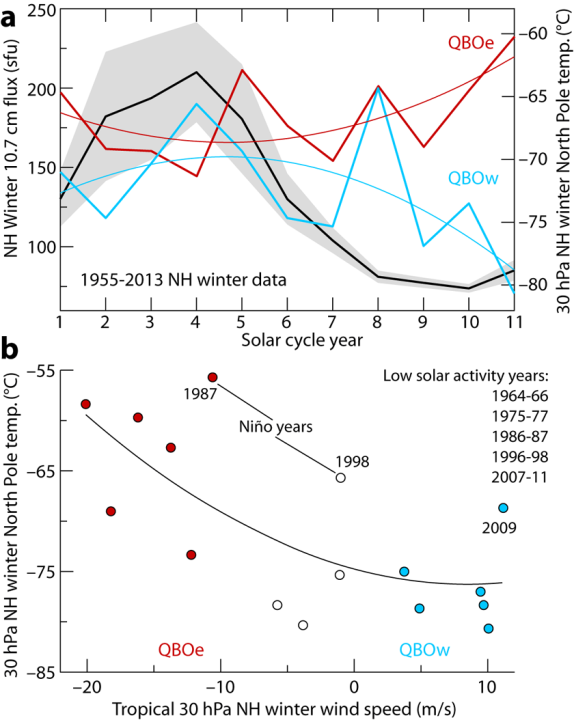
Fig. 2.3 reveals the impact of photo voltaic exercise on winter North Pole stratospheric temperature. In panel (a) the black curve and light-weight gray space present the winter (DJF) 10.7 cm flux common and customary deviation between Dec. 1955 and Feb. 2013. It’s a proxy for photo voltaic exercise, adjusted to an 11-year photo voltaic cycle. The coloured curves correspond to winter temperature at 30 hPa (stratosphere) over the North Pole calculated as the common of the three extra central values amongst DJFM month-to-month common temperatures (outlier discarded) and plotted in accordance with the place within the 11-year photo voltaic cycle. The dark-red thick curve is the temperature for winters when the QBO offered common DJF values decrease than –5.8 ms–1 (adverse values denote easterly wind) akin to QBOe (easterly). Darkish-red skinny curve is the quadratic regression. Gentle-blue thick curve is the temperature for winters when the QBO offered common DJF values larger than 1.1 ms–1 (optimistic values denote westerly wind) akin to QBOw (westerly). The sunshine-blue skinny curve is the quadratic regression.
Fig. 2.3 panel (b) is a scatter plot of 30 hPa winter North Pole temperature, decided as in (a) versus tropical 30 hPa winter wind velocity, for years with very low photo voltaic exercise, akin to years 9 to 11 within the photo voltaic cycle as outlined in (a), and indicated within the graph. Darkish-red-filled dots are QBOe/temperature values used for a similar coloration curve in (a). Gentle-blue-filled dots are QBOw/temperature values used for a similar coloration curve in (a). Black skinny curve is the quadratic regression. Sturdy El Niño years are labeled. The open circles are intervals of low to barely adverse (easterly) wind velocity. Knowledge on North Pole stratospheric temperature is from the Institute of Meteorology on the Freie Universität Berlin. Knowledge on the ten.7 cm photo voltaic flux is from the Royal Observatory of Belgium STAFF viewer.
In keeping with Peixoto and Oort’s (1992) essential e book Physics of Local weather, the unusually excessive correlation between photo voltaic exercise and sea-level strain or floor temperature over intensive areas of the NH, when the QBO section is taken into account, seem to elucidate an essential fraction of the full interannual variability within the winter circulation. However photo voltaic exercise isn’t the one issue affecting polar vortex power, it additionally is determined by the QBO by means of the Holton-Tan impact (see Half I, Sect. 1.6) and on El Niño/Southern Oscillation (ENSO). El Niño years destabilize the vortex, and tropical volcanic eruptions stabilize the vortex which produces a hotter northern mid-high latitude winter.
Since Peixoto and Oort (1992), fashionable climatology seems to have forgotten in regards to the essential photo voltaic impact on the polar vortex and winter circulation. Dennis Hartmann’s World Bodily Climatology (2nd ed. 2016) doesn’t point out Labitzke or her discovering of a photo voltaic impact on winter circulation, and even fails to say the polar vortex (not within the topic index). Surprisingly, it’s the similar scenario with the extra specialised An Introduction to Dynamic Meteorology (5th ed. Holton & Hakim 2013). Let’s keep in mind that James Holton (1982) reviewed the doable bodily mechanisms of photo voltaic variability’s impact on local weather through dynamic atmospheric coupling, so it isn’t as if he didn’t find out about it. Fashionable climatology is intentionally ignoring recognized proof of a sun-climate impact.
2.4 Results on El Niño/Southern Oscillation
The photo voltaic impact on ENSO can be ignored by fashionable climatology. A latest assessment on ENSO complexity by 45 outstanding ENSO consultants (Timmermann et al. 2018) fully fails to say any photo voltaic implication regardless of the ample bibliography on the topic (Anderson 1990; Landscheidt 2000; White & Liu 2008; Wang et al. 2020; Leamon et al. 2021; Lin et al. 2021). Deser et al. (2010) analyze the facility spectrum of the Niño-3.4 (5°N–5°S, 170–120°W) SST time collection and solely point out the two.5–8 years vary, fully ignoring the distinct 11-yr peak within the collection (Fig. 2.4b).
One of many authors (JV) lately studied the affiliation between growing photo voltaic exercise and La Niña situations within the Niño-3.4 area Oceanic Niño Index (ONI). A Monte Carlo evaluation confirmed that the La Niña occurrences, which came about throughout instances of rising photo voltaic exercise (from 35 to 80 % of the ascending section of the photo voltaic cycle), between 1950–2018, have solely a 0.7% likelihood of being attributable to probability, demonstrating that ENSO is modulated by photo voltaic exercise (Vinós 2019; 2022). The latest La Niña situations since 2020 after the December 2019 photo voltaic minimal can solely have decreased the already low likelihood that the affiliation is because of probability.
The solar-ENSO modulation is uncovered by a easy frequency evaluation of ENSO modes. ENSO shows three temporal modes: El Niño (heat mode), La Niña (cool mode), and Impartial. The ENSO system is often thought-about to be an oscillation between El Niño and La Niña modes attributable to their opposing temperatures. This view seems to be incorrect. NOAA’s Local weather Prediction Heart classifies ENSO winter modes (yr akin to January) in accordance with SST knowledge within the Niño-3.4 area (Domeisen et al. 2019). Utilizing this classification, it’s trivial to reveal that La Niña years strongly anti-correlate to Impartial years, not El Niño years (Fig. 2.4a) for the 1960–2020 interval (1962–2018 proven utilizing a gaussian filter).
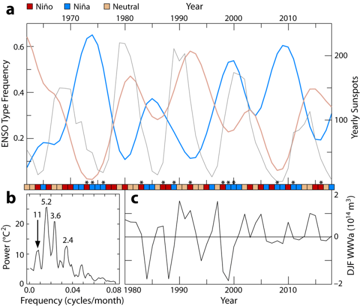
In Fig. 2.4, (a) is the frequency of Niña years (medium blue thick line) and Impartial years (mild brown thick line) in a 5-year centered shifting common (gaussian filtered) between 1962–2018 displaying an virtually good anti-correlation for your complete interval. The small containers alongside the underside are the ENSO mode classification after Domeisen et al. 2019, with darkish purple containers for Niño years, and colours matching the curves for Niña and Impartial years. Asterisks mark robust Niño and Niña occasions with ≥1 °C anomaly in Oceanic Niño Index. The positive gray line is the variety of yearly sunspots.
Fig. 2.4 panel (b) is the facility spectrum of the 1900–2008 Niño-3.4 SST anomaly time collection after Deser et al. 2010. An arrow marks the 11-year frequency peak which may correspond to the photo voltaic cycle impact. Panel (c) is the Dec–Feb common heat water quantity anomaly above the 20 °C isotherm between 5°N–5°S, 120°E–80°W. The information is from the TAO Challenge Workplace of NOAA/PMEL.
Los Niños sometimes happen each 2–3 years (vary 1–4 years), so there are all the time 1–3 Niños in a 5-year interval. La Niña and Impartial years are extra variable, as there may be 0–4 of every in a 5-year interval. The robust anti-correlation between La Niña and Impartial years signifies ENSO has been profoundly misunderstood and even its naming is inaccurate, appropriately La Niña/Southern Oscillation. Evaluation of the nice and cozy water quantity within the equatorial Pacific (Fig. 2.4c) signifies that vitality tends to build up throughout Niña years, and it’s launched throughout Niño years, with Impartial years someplace in between. Vitality tends to build up within the equatorial Pacific, one of many main photo voltaic vitality entry factors into the local weather system. The ENSO system oscillates between accumulation (Niña years) and inefficient distribution (Impartial years). When the system accumulates extra vitality, Los Niños happen to effectively unfold the surplus by means of the remainder of the local weather system.
The La Niña/Impartial oscillation is section locked to the photo voltaic cycle (Fig. 2.4a). El Niño frequency can be affected by the photo voltaic cycle, as different authors have famous (Landscheidt 2000), however not so strongly, and the incidence of Niño years barely perturbs the Niña/Impartial match to the photo voltaic cycle. This photo voltaic impact on ENSO explains the 11-year frequency peak within the Niño-3.4 SST energy spectrum. It additionally explains why multidecadal intervals of excessive photo voltaic exercise, like the fashionable photo voltaic most, are inclined to show much less Niñas, and why the interval of decreased photo voltaic exercise since 1998 has displayed extra frequent Niñas with much less adverse heat water quantity anomaly values. Coinciding with the Pause in world warming, heat water quantity anomalies have considerably fewer adverse values, reaching lower than one fourth of earlier adverse values (Fig. 2.4c). El Niño is the odd one out within the Niña/Impartial oscillation, which explains why El Niño is available in totally different flavors (Central Pacific versus Jap Pacific) and shows an unlimited variability in the course of the Holocene (Moy et al. 2002), with Niño exercise very decreased in the course of the Holocene Climatic Optimum. El Niño taste, frequency, and depth reply to the necessities of the poleward meridional vitality transport course of.
One can solely surprise that, if fashionable climatology wasn’t so blind to the sun-climate impact, the photo voltaic modulation of ENSO could be frequent information and mentioned in critiques like Timmermann et al. (2018) and Domeisen et al. (2019). It’s embarrassing, and a sign that fashionable climatology has misplaced its method, that it has taken a molecular biologist to note.
2.5 Results on Earth rotation
Photo voltaic exercise impacts the Earth’s velocity of rotation. The impact is small, however it has been measured for the reason that introduction of atomic clocks within the late Nineteen Fifties. This photo voltaic impact has been seen periodically by researchers, reported, ignored, and forgotten, solely to be seen once more by one other researcher believing it was an authentic discovery. The primary report seems to be by René Danjon in 1962. In 1971 Rodney Challinor, with 14 years of information, associated the annual modifications within the size of day (LOD) to the sunspot cycle. He recommended that modifications within the world atmospheric circulation induced by photo voltaic exercise modifications is perhaps answerable for the impact on Earth’s rotation price (Challinor 1971). Jan Vondrák (1977) and Robert Currie (1980) additionally rediscovered the solar-Earth rotation relationship. Within the Nineties Daniel Gambis (Gambis & Bourget 1993) and within the 2000s Rodrigo Abarca del Río (Abarca del Río et al. 2003) continued the research on the solar-Earth rotation relationship. Extra lately Le Mouël et al. (2010) and Barlyaeva et al. (2014) investigated doable mechanisms of this relationship.
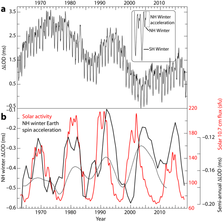
In Fig 2.5 (a) the month-to-month ΔLOD for the 1962–2018 interval is plotted. The inset reveals two years of information with 4 semi–annual elements akin to northern (NH) and Southern Hemisphere (SH) winters. The panel (b) black curve is the 3-point smoothed amplitude of the NH winter change in ΔLOD from weekly knowledge after 31-day smoothing. Decrease values point out a bigger change in Earth’s rotation velocity. The purple curve (proper scale) is photo voltaic exercise as decided by 10.7 cm flux (photo voltaic flux items, gaussian smoothed). The dotted curve (proper scale) is a Quick Fourier Rework with a 4-year window of the time spinoff 0.5-yr part of LOD, 30-month smoothed, after Barlyaeva et al. 2014.
It has been demonstrated that, for intervals of time between 14 days and 4 years, modifications within the atmospheric angular momentum (AAM) of the troposphere and stratosphere account for over 90% of the modifications in LOD (Rosen & Salstein 1985), because the Earth’s rotation price should regulate to maintain the full momentum of the Earth system fixed. Seasonal variation in ∆LOD has been recognized for many years to mirror modifications in zonal circulation (Lambeck & Cazennave 1973). For a dialogue of zonal winds, largely from UCLA, see right here. The biennial part of ∆LOD displays modifications within the QBO (Lambeck & Hopgood 1981), whereas the three–4-year part matches the ENSO sign (Haas & Scherneck 2004). The 2015–16 El Niño produced a ∆LOD tour reaching 0.81 ms in January 2016. A really shut match between the semi-annual part in ∆LOD and photo voltaic exercise shouldn’t be anticipated given these different causal brokers.
The hyperlink between modifications in ΔLOD, modifications in AAM, and photo voltaic variability may be very simple, and essentially should go within the route “photo voltaic → ambiance → rotation.” The momentum of the Earth system is conserved on the scales concerned and it isn’t doable that modifications within the velocity of rotation of the Earth have an effect on photo voltaic exercise. A relationship between multidecadal modifications in ΔLOD and modifications in local weather was proposed by Lambeck and Cazenave (1976). With out contemplating a photo voltaic implication, they reported on the similarity between the tendencies of quite a few local weather indices for the previous two centuries and modifications in ∆LOD. Particularly, Lambeck and Cazenave famous that LOD variations correlate nicely with world temperature and floor strain, each of that are indicators of worldwide wind circulation. They concluded that intervals of accelerating zonal winds correlate with accelerating Earth rotation whereas intervals of reducing zonal circulation correlate with deceleration. They discovered a lag of 5–10 years within the climatic indices. Their outcome has been reproduced a number of instances (e.g., Mazzarella 2013).
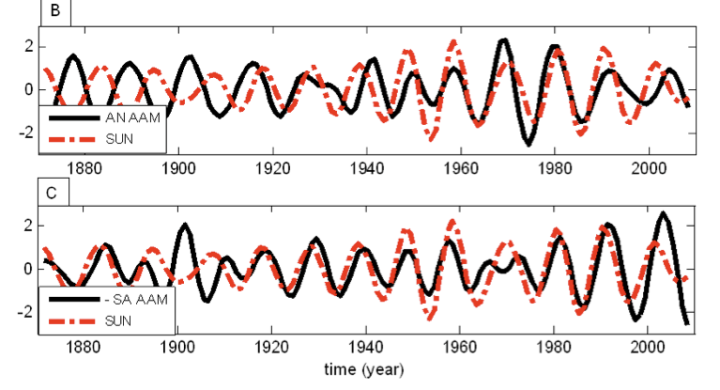
The AAM may be reconstructed again to 1870, and its decadal modifications within the annual and semiannual elements (associated to the annual and semiannual elements of ∆LOD) show a correlation with the 11-yr photo voltaic cycle. Apparently the correlation between the annual part and the sunspot quantity underwent a section shift c. 1920 (Fig. 2.6B). It is a time when a number of sun-climate correlations inverted (see Half I, Fig. 1.3), discrediting sun-climate correlation research. We have no idea what causes these inversions within the local weather response to photo voltaic exercise and possibly we is not going to know till a brand new inversion takes place, since we have to know what occurs within the stratosphere throughout them. They seem to happen each 80–120 years (Hoyt & Schatten 1997). Nevertheless, we are able to conclude two essential issues from the existence of those sun-climate inversions. First, that photo voltaic exercise impacts local weather by means of its impact on atmospheric circulation (AAM), not by means of variations in whole irradiance. And second, when the photo voltaic impact on the annual part of the AAM shifts phases, the photo voltaic impact sample on floor temperature and precipitation inverts. The simultaneous incidence of the section shift in AAM (Earth rotation) and the sun-climate sample inversion at c. 1920 demonstrates that these shifts are an intrinsic characteristic of the sun-climate impact.
For the reason that photo voltaic impact on Earth’s rotation price and world atmospheric circulation are intentionally ignored by fashionable climatology, they aren’t included usually circulation fashions. This enables the IPCC to wrongly conclude that photo voltaic variability has no important impact on local weather change since 1850. The truth, nevertheless, is that a terrific a part of the local weather change that has taken place in the course of the 20th century has been because of the fashionable photo voltaic most.
2.6 Results on planetary waves
In 1974, Colin Hines proposed that the sun-climate impact may very well be completed by modulating the planetary waves propagation properties of the ambiance, and James Holton agreed that such mechanism was viable, however objected that little proof existed for it on the time (Hines 1974; Holton 1982). This was not fully appropriate. Geller and Alpert (1980) not solely demonstrated the viability of the Hines mechanism however confirmed that modifications within the solar’s ultraviolet (UV) emissions, by altering the stratospheric thermal construction, may very well be answerable for modifications within the imply zonal wind, leading to inter-annual variations in stationary planetary wave patterns that might induce very important modifications in regional local weather. Their modeling outcomes not solely quantified the magnitude of the anticipated results however indicated that the tropospheric planetary wave response to solar-induced modifications within the zonal imply state of the stratosphere must be regional, very evident at some longitudes and latitudes, and absent in others (Fig. 2.2).
Waves within the ambiance (Fig. 2.7) are oscillatory motions that outcome from a stability between the inertia of a parcel of air that has been set in movement and a restoring pressure. These oscillatory motions produce periodic modifications in atmospheric variables (strain, geopotential peak, temperature, or wind velocity) which will stay stationary or propagate horizontally or vertically. Atmospheric waves transmit vitality and momentum with out materials transport of air parcels to distant areas on time scales a lot shorter than the transit time for air parcels. The momentum and vitality are fed into the background circulation because the wave dissipates or breaks, altering it. Most climate disturbances are related to a number of kinds of atmospheric wave (Holton 2003).
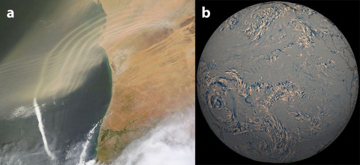
In Fig. 2.7, (a) is a photograph of atmospheric waves made seen by Saharan mud off the northwestern coast of Africa. The photograph is from NASA. Picture (b) are of atmospheric waves attributable to the Tonga 2022 eruption that circled the globe. The photograph was captured by NOAA’s GOES-West satellite tv for pc IR channel. Tonga is positioned on the backside left of the picture. From Mathew Barlow and after Duncombe (2022).
Vertically propagating planetary (Rossby-Haurwitz) waves are generated by circulation over continental-scale topography, by continent–ocean heating contrasts, and by nonlinear interactions amongst transient tropospheric wave disturbances. Their restoring pressure is the potential vorticity latitudinal gradient induced by the Coriolis parameter attributable to planetary rotation. Planetary waves zonal wavenumber is an integer designating the variety of waves round a latitude circle, thus at 60° a wavenumber 1 planetary wave has c. 12,000 km meridional scale. The vertical propagation of stationary planetary waves requires the presence of imply westerly winds of velocity decrease than a essential worth, in what is called the Charney–Drazin criterion. In observe, zonal wavenumbers 1–3 account for over 96% of wave propagation into the extratropical stratosphere, and this occurs solely within the winter hemisphere.
Small modifications in photo voltaic UV vitality could cause huge modifications within the vitality and momentum delivered by planetary waves to the stratosphere. These are then mirrored in modifications within the troposphere, by means of stratosphere-troposphere coupling, as recommended by Hines (1974), and proven by Geller and Alpert (1980). This course of constitutes the idea of the “top-down” mechanism of sun-climate impact. This course of or mechanism bypasses the issue of the small change in photo voltaic vitality output in the course of the photo voltaic cycle, because the vitality to have an effect on local weather is offered by planetary waves, which alter the worldwide atmospheric circulation in regionally various patterns. Kodera and Kuroda (2002) confirmed that with the arrival of winter, the stratospheric circulation modifications from a radiatively managed state to a dynamically managed state, and the transition is modulated by photo voltaic exercise, with the photo voltaic most prolonging the radiatively managed state. This modulation impacts the power of the stratospheric sub-tropical and polar evening jets, and the Brewer–Dobson circulation.

Perlwitz and Harnik (2003) offered proof that planetary waves mirrored within the stratosphere on sure winters had a tropospheric impact. Nathan et al. (2011) confirmed that the zonally uneven ozone area was crucial in mediating the results of photo voltaic variability on the wave-driven circulation within the stratosphere. The research of planetary waves within the stratosphere is latest and tough to hold out. Powell and Xu (2011), utilizing two reanalysis datasets and satellite tv for pc microwave sounding unit observations, constructed a planetary wave amplitude index for the 55–75°N stratosphere and confirmed it was related to the Arctic Oscillation. They discovered substantial shifts within the stratospheric state attributable to modifications in wave amplitude and sample anomalies. The principle ones had been related to a 2-year oscillation that was in section with the photo voltaic cycle. Throughout photo voltaic maxima planetary wave amplitude was decreased, whereas throughout photo voltaic minima modifications within the meridional temperature gradient and vertical wind shear result in a rise in planetary wave amplitude (Fig. 2.8). The detected photo voltaic cycle impact might account for 25% of the variability in wave amplitude (Powell & Xu 2011).
The Powell and Xu (2011) discovering offers direct observational proof for the Geller and Alpert (1980) research. Of their research, Geller and Alpert confirmed {that a} 20% change within the imply zonal circulation at 35 km peak or decrease could be the required order of magnitude to supply the noticed interannual variability within the tropospheric wave sample at center and excessive latitudes. The discovering by Powell and Xu that the photo voltaic impact would possibly clarify 25% of stratospheric wave amplitude signifies that the UV photo voltaic impact, coupled with ozone variability, can clarify the essential sun-climate impact on winter atmospheric circulation first detected by Labitzke and van Loon (1988).
2.7 Conclusion
This half (2nd of the collection) demonstrates the existence of a wealth of data in regards to the sun-climate impact, laboriously produced by scientists who haven’t acquired correct credit score for shining mild on what might be essentially the most advanced, most controversial drawback in climatology. This information offers adequate clues in regards to the sun-climate impact mechanism.
It’s now not acceptable to say that photo voltaic variability in whole irradiance is simply too small to have a major impact on local weather, when there may be a lot proof that variations in whole irradiance are usually not how photo voltaic variability primarily impacts local weather.
It’s now not acceptable to say that oblique results of photo voltaic variability are too unsure since their mechanism is unknown when clear proof for the mechanism is revealed and ignored.
It’s now not acceptable to solely contemplate modifications in whole irradiance in mannequin research after which declare that the fashionable photo voltaic most didn’t contribute to fashionable world warming.
It’s now not acceptable to reject a sun-climate impact based mostly on the dearth of a easy correspondence between floor temperature and photo voltaic exercise, when proof means that the photo voltaic impact on local weather works by means of modifications in atmospheric circulation.
If it stays acceptable, then we’re constructing the foundations of local weather change science on a false premise that forestalls us from understanding it. It would set again the scientific development of climatology by a long time, simply because the refusal to simply accept the proof for continental drift set geology again 4 a long time. And it’ll have large repercussions for the fame of science, as most climatologists present a justification for costly socioeconomic insurance policies whereas ignoring an essential, well-documented, solar-climate connection.
The bibliography may be downloaded right here.
A listing of abbreviations used may be downloaded right here.
This publish was first revealed on Local weather And so on.
